
A generalized linear model has three basic components:
- Random Component: Identifies The response variable and its probability distribution.
- Systematic Component: Specifies the explanatory variables (independent or Predictors) used in the linear predictor function.
- Link Function: Is a function of the expected value of Y, E (Y), as a combination linear of the Predictor variables.
Random Component
The random component of a GLM consists of a random variable with independent observations ![]()
In many applications, Y observations are binary and identified as success and failure. Although in a more general way, each Yi It indicates the number of successes of between a fixed number of trials and is modeled as a binomial distribution.
At other times each observation is a count, which can be assigned to and a Poisson distribution or a negative binomial distribution. Finally, if the observations are continuous can be assumed for and a normal distribution.
All these models can be included within the so-called exponential family of distributions so that Q (θ) receives the name of natural parameter
Systematic Component
The systematic component of a GLM specifies the explanatory variables, which enter in the form of fixed effects in a linear model, that is to say, the variables ![]() are related by
are related by
Esta combinaci´on lineal de variables explicativas se denomina predictor lineal. Alternativamente, se puede expresar como un vector ![]() such as
such as
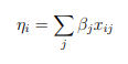
Where ![]() It is the value of the J-th Predictor in the i-th individual, and i = 1,…, N. The Independent term α is obtendrıa with this notation making all the
It is the value of the J-th Predictor in the i-th individual, and i = 1,…, N. The Independent term α is obtendrıa with this notation making all the ![]() are equal to 1 for all i.
are equal to 1 for all i.
In any case, you can consider variables that are based on other variables such as ![]() or
or ![]() to model interactions between variables or effects curved linear
to model interactions between variables or effects curved linear ![]() .
.
Link Function
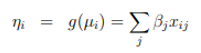
The expected value of Y Is denoted as Μ = E (Y), then the link function specifies a function g (•) that relates µ with the linear predictor as
Thus, the function link g (•) relates the components random and systematic.
So, for i = 1,…, N,
The simplest g function is g (µ) = Μ, that is, the identity that gives rise to the model of classic linear regression
Typical linear regression models for continuous answers are a particular case of the GLM. These models generalize the ordinary regression in two ways: allowing and have different distributions than normal and, on the other hand, including different link functions of the media. This is quite useful for categorical data.
The GLM models allow the unification of a wide variety of estadısticos methods such as regression, ANOVA models and categorical data models. The same algorithm is actually used to obtain maximum likelihood estimators in all cases. This algorithm is the basis of the GENMOD procedure of SAS and the GLM function of R.
Generalized Linear Models for Binary Data
In Many cases the answers have only two categorıas of the type yes/no so that you can define a variable and take two possible values 1 (success) and 0 (failure), it is say Y ∼ Bin (1, π). In this case with ![]()
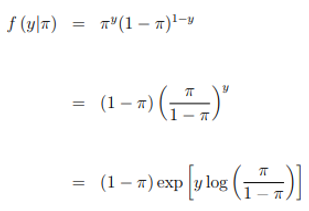
The Natural parameter is
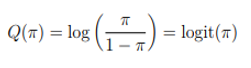
In this case
dependent on p explanatory variables
In binary responses, an analog model to linear regression is ![]()
Which is called a linear probability model, because the probability of success changes linearly with respect to ![]()
The β parameter represents the change in probability per unit of ![]() . This model is a GLM with a binomial random component and with link function equal to the identity.
. This model is a GLM with a binomial random component and with link function equal to the identity.
However, this model has the problem that although the odds should be between 0 and 1, the model can sometimes predict values
Example
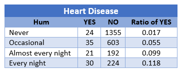
You have the following table where you choose several levels of snoring and put in relationship to heart disease. The values {0, 2, 4, 5} are taken as relative ratings of snoring.
You get
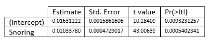
In other words, the model you get is
For example, for people who do not snore ![]() the estimated probability of disease cardiac will be
the estimated probability of disease cardiac will be ![]()