
Statistically speaking, Design of Experiments (DoE) deals with planning, executing, analyzing, explaining and even predicting (by a mathematical model) the behavior of a phenomenon, after performing trials under controlled conditions. These trials evaluate:
• All the variables immersed in the phenomenon (which in DoE, we will call factors).
• Interactions, if any present, among factors.
• Factors that mainly (or, statistically speaking, significantly) impact, affect or rule on the phenomenon.
On the traditional basis, a trial-and-fail analysis would help us defining the best way of adjusting a machine, improving a dish (in the kitchen, why not?), creating the lightbulb (as Edison did) or selecting the best amount of a component for an I.V. mixture. However, this unidimensional approach is time costing and would not allow us obtaining the best (the optimal) approach.
If we want to run faster, we need to use statistics, and this is where DoE comes to play. Taking as backup concepts like confident intervals, hypothesis tests and ANOVA, DoE is a powerful tool for identifying in faster time and reasonable costs the optimum zone for a process or product.
An experiment (again, in DoE language), according to Douglas C Montgomery in his classic book Design and Analysis of Experiments, is a trial or series of trials on which process or system input variables are modified to output responses can be observed and defined.
In other words, if we want to study and comprehend a phenomenon, anyone, we need to set which variables (factors) would impact its behavior and in which extent. Then, delimit the zone (boundaries) where we want to evaluate these variables (low and high boundaries or levels) and then, perform trials combining factors and levels among them (running the experiments). The results obtained (responses) are statistically analyzed and, in some cases, a predicting mathematical model can be achieved. If we know which the best responses are we want to obtain, an optimal zone can be defined after these results.
There are several DoE models to be used. For lean sigma purposes, most used is factorial 2k, where k is factors number.
Currently, there is many software commercially available, such as Quantum XL, Minitab, Design-Expert, Unscrambler X, JMP and many, many more. All of them are quite good for factorial DoE. Selection depends on how more complex analysis you need to perform or if you need to use more complexes models.
Now, let’s show how factorial DoE works for defining main variables that affect a process and a first optimization zone may be achieved.
Let’s assume we have a machine that produces slugs. We need to assure slugs meet specification of target weight ± 5%.
Also, we know that for the machine, three main factors may impact on the weight variation: previous pressure, penetration height and feeding speed. The minimum and maximum values for the adjustment of each one of the factors have been defined after previous trials and are shown in the following table. Levels -1 and +1 are used to express in a simplest way lower and higher values for further statistical analysis and are called coded values.
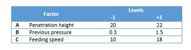
Finally, we absolutely want productivity. So, we need assure that best adjustment is gotten at the best machine speed: 250,000 slugs/h (80% of the design speed of the machine). This will be a fixed speed for all the trials.
As we define 3 variables (or factors, or 3 k’s), our design is a factorial 23, which means that we are trying 3 factors (exponential value) at two levels (base number): low (-1) and high (+1).
If we mix levels low and high among the three factors, we obtain 8 different combinations. We can observe that 23 = 8.
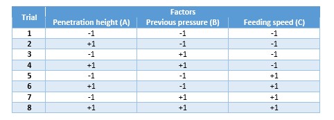
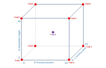
Hard to understand in a table? Ok, we can check this also in a visual way. Let’s assume each of the factors are axis of a 3D chart. We can draw a cube and using each point as our initial test zone. Can you see now why coded values are useful?
But there is more: do you want extra information? We can include an extra trial using middle values of each level. So, we get a ninth trial, which will be coded as (0,0,0). In the chart you can identify it with the purple point.
Finally, what are we going to measure? Our response must give us a good certainty grade that weight variation meets specification. This index is not more than process capability, CP.
Now that everything is ready, we need to run our experiments, got data and analyze. Which we will do in our next article.