
Comparing data samples and variances.
Smart business involves a continued effort to gather and analyze data across a number of areas. One of those key areas is how certain events affect business staff, production, public opinion, customer satisfaction, and much more. The Analysis of Variance (ANOVA) method assists in analyzing how events affect business or production and how major the impact of those events is. It determines if a change in one area is the cause for changes in another area.
Data Groups & Variances
To analyze if one change of events is the cause for another change, multiple factors must be accounted for. Variances within each sample group of data and variances between the set of groups of data must be analyzed. We must take into account, for example, differences in skill sets within each group of people surveyed. This is done by calculating the mean (or average) of each group. We must also watch for changes in results between each group of people. This is done by taking the mean of each group’s mean. This will make more sense as we work through an example.
There are different methods for analyzing variances depending on your sample data and how many variances there are. For this introductory explanation, we will be working through a subset of ANOVA called the F-Test using three groups of sample data and two types of variances between them–type of drink consumed and change in productivity.
Our Example Scenario
You run an accounting firm and want to conduct a productivity test. You seek to discover if different beverages consumed by your staff throughout the day affect productivity. More specifically, you want to know if the beverages affect how quickly your accountants complete a financial transaction research project. You will be conducting the test among fifteen accountants who will all be given the same assignment with 50 transactions to reconcile. The accountants will be in 3 groups of 5.
Group 1 will be given soda.
Group 2 will be given a B-vitamin drink.
Group 3 will be given coffee.
For the F-Test, we are trying to prove that something is not true. To look at it another way, we are attempting to prove that there is no relation between two variances. In this scenario we will seek to prove the following statement true. The statement below is called the Null Hypothesis, or H0:
H0 = “The type of beverage consumed by accountants has no bearing on how productive they are.”
If the F-Test proves that the beverages have no effect on productivity, we will accept the null hypothesis. If the beverages do affect productivity, we will reject the null hypothesis.
Variance Calculation – Step-by-Step
Over the course of two days, you have tracked how many hours it took each of your fifteen staff members to complete the same assignment. Here are the results: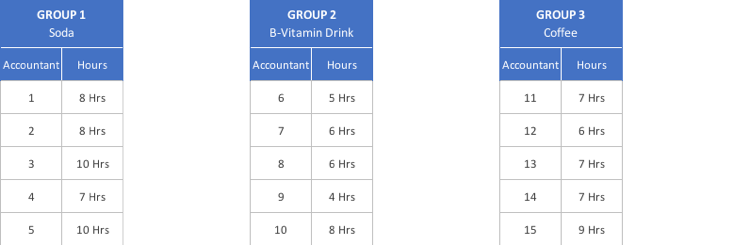
To determine if the supplied beverages affect productivity, we will be working with the following calculation:
Total Sum of Squares (SST) = Sum of Squares Between Groups (SSB) + Sum of Squares Within Groups (SSW)
Sum of Squares Within Groups (SSW)
Our first calculation, the Sum of Squares Within Groups or SSW, is used to determine if variation in productivity has anything to do with variances between people within each group:

In this example, some accountants are just faster than others on a normal basis. Looking at Group 1, you can see that two accountants take ten hours to complete the assignment while another takes only 7.
To calculate Sum of Squares Within Groups (SSW):
- Add the total hours for each group together and find the mean (average) for each group:
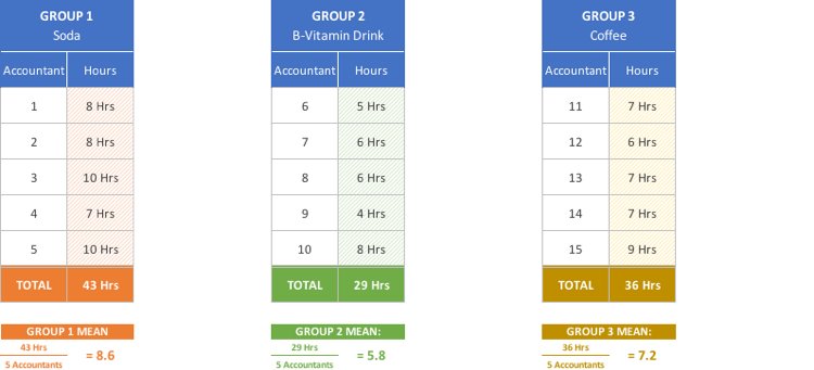
- Subtract the mean for each group from the observation (hours in this case) for each member of the group and square each result. This is the sum of squares for each individual group:
( Observation – Mean ) 2
Now we can find our Sum of Squares Within Groups (SSW). To do so, simply add the sum of squares for each group together:
SSW = Group 1 Sum of Squares + Group 2 Sum of Squares + Group 3 Sum of Squares
SSW = 7.2 + 8.8 + 4.8 = 20.8
Total Sum of Squares (SST)
The next part of our formula that we will calculate is the Total Sum of Squares, or SST. To do so, we will perform the same calculations as above, but will do so upon the entire group. We will treat the entire population of the study–all fifteen accountants–as one large group.
- Calculate the mean for the entire population:
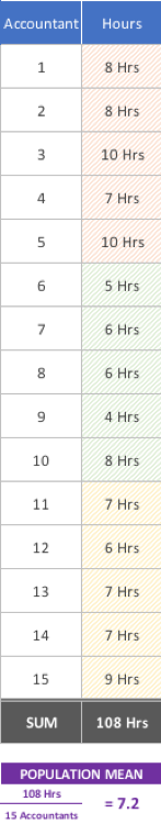
Subtract the mean for the entire population from the observation (hours) for each member of the group and square each result:

The sum we obtain is our Total Sum of Squares (SST):
SST = 40.4
Sum of Squares Between Groups (SSB)
As you can see in our formula below, we now have two of the three values needed:
Total Sum of Squares (SST) = Sum of Squares Between Groups (SSB) + Sum of Squares Within Groups (SSW)
40.4 = Sum of Squares Between Groups (SSB) + 20.8
We could, at this point, use algebra to find SSB. However, we will go through the calculation of it for the sake of deeper understanding.
- Subtract the mean for the entire population from the mean of each sample group:
Group 1 Mean – Population Mean 8.6 – 7.2 = 1.4
Group 2 Mean – Population Mean 5.8 – 7.2 = -1.4
Group 3 Mean – Population Mean 7.2 – 7.2 = 0.0
- Square each result:
1.42 = 1.96
-1.42 = 1.96
0.02 = 0.00
- Add the squared results together:
1.96 + 1.96 + 0.00 = 3.92
- Multiply this result by the number of observations (accountants) in each group, which are five:
3.92 x 5 = 19.6
This result is our Sum of Squares Between Groups (SSB):
SSB = 19.6
Final Formula
Plugging the three values we calculated into our formula, here is what we get:
Total Sum of Squares (SST) = Sum of Squares Between Groups (SSB) + Sum of Squares Within Groups (SSW)
ß
40.4 = 19.6 + 20.8
Final Calculations
Now, we can begin our final calculations:
SSB Divided by its Degrees of Freedom
| Sum of Squares Between Groups |
| Degrees of Freedom |
Degrees of Freedom for SSB is the number of groups minus one. With 3 groups, the degrees of freedom is 3 – 1, which is 2:
| Sum of Squares Between Groups | = | 19.6 | = 9.8 |
| Degrees of Freedom | 2 |
SSW Divided by its Degrees of Freedom
| Sum of Squares Within Groups |
| Degrees of Freedom |
Degrees of Freedom for SSW is the total number of observations minus the number of groups. With 15 total observations and three groups, the degrees of freedom is 15 – 3, which is 12:
| Sum of Squares Within Groups | = | 20.8 | = 1.73 |
| Degrees of Freedom | 12 |
F-Statistic / F-Ratio
The F-Statistic (also called the F-Ratio because it is a ratio) is calculated by dividing the larger result above by the smaller result:
| F | = | 9.8 | = 5.65 |
| 1.73 |
Critical Value
Our last calculation is the Critical Value, which is used to determine whether or not to reject or accept our Null Hypothesis (H0). For our two-variance test, if our F falls below the Critical Value, this means that the beverages consumed by accountants do not affect productivity and we accept the Null Hypothesis. If it falls above, then the beverages do affect productivity and we reject the Null Hypothesis.
To find the Critical Value, we look up the degrees of freedom for the numerator and denominator of our F-Ratio above in a table called an F-Distribution Table. There are different tables you can use depending on various factors, but we will not cover that here. Look up the numerator degrees of freedom in the column header of the table and denominator degrees of freedom in the row header. Find where they intersect and that is your Critical Value. The degrees of freedom for our numerator was 2, and for our denominator was 12:
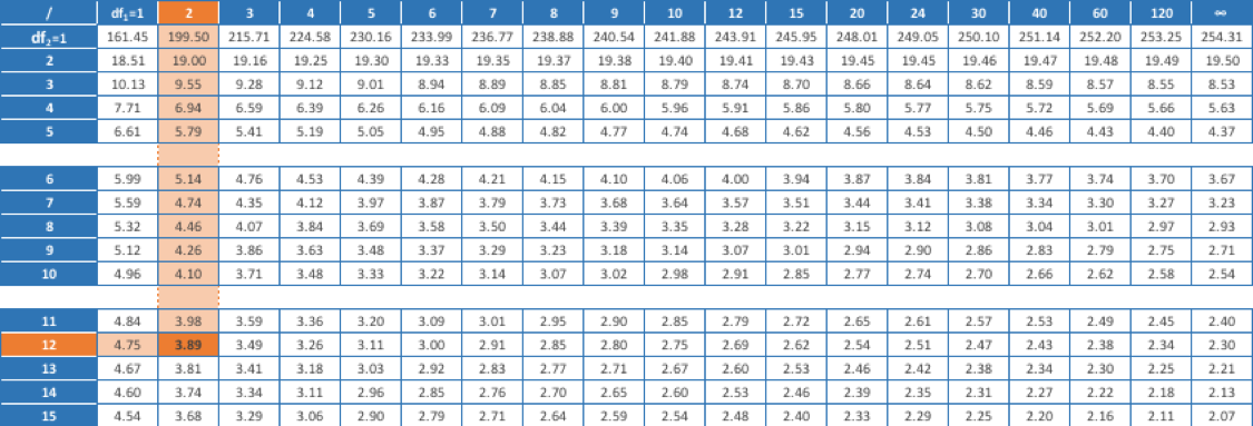
Critical Value = 3.89
Final Steps
Lastly, we plug our F-Ratio and our Critical Value into a statistical distribution chart. As you can see, the F-Ratio falls above the Critical Value. As stated prior, this means that we reject our Null Hypothesis that the beverages have no effect on accountant productivity:
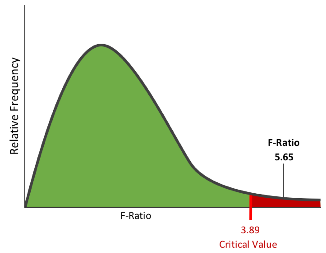
Therefore:
H0 = “The type of beverage consumed by accountants has no bearing on how productive they are.” = FALSE
The beverages do have an effect on accountant productivity.